Blood Flow Modelling
Vascular diseases, such as stenosis and aneurysms, are often associated with changes in blood flow patterns and the distribution of wall shear stress (WSS). Modelling and analysis of the hemodynamics in the human vascular system improve our understanding of vascular disease, and provide valuable insights, which can help in the development of efficient treatment methods. In recent years, computational methods have been widely used for patient-specific modelling of blood flow in vascular structures. However, there has been limited applications of computational hemodynamics in clinical practice.
In this work, a robust and semi-automatic modelling pipeline for blood flow through subject-specific arterial geometries is presented. The framework consists of image segmentation, domain discretization (mesh generation) and computational fluid dynamics. All the three subtopics of the pipeline are explained using an example of flow through a severely stenosed human carotid artery.
Proposed Pipeline
- Applied a 3D segmentation method based on a geometrical potential force (GPF) to reconstruct the vascular geometries;
- Employ an automatic voxel thinning procedure to obtain the axes of the vessel and vessel branches;
- Use the level set functions obtained from the 3D image segmentation method to generate valid surface meshing;
- The surface mesh generation is followed by an automatic procedure to construct the boundary layer mesh on the inner surface of the vessel walls;
- The volume mesh, based on the Delaunay method, is then used to complete the mesh generation step;
- Once the mesh is finalized, the flow boundary conditions are decided based on either available flow measurements or assumed flow rate;
- Once the boundary conditions are determined, the flow solver (a finite element solver) is used to determine the flow and wall quantity distributions, both with respect to time and space.
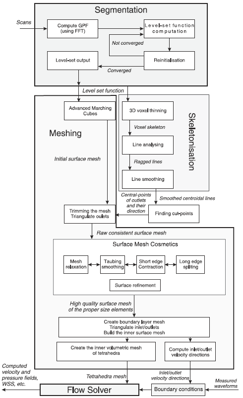 |
| Flowchart of the proposed pipeline. |
Blood Vessel Geometry Extraction
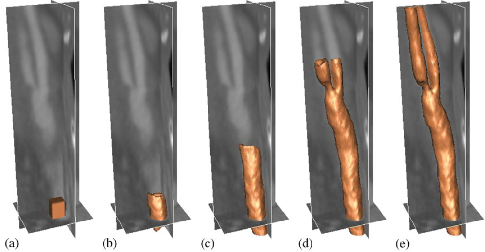 |
| Segmentation of a carotid artery using GPF-based deformable model: (a) initial surface, (b) after 11, (c) after 81, (d) after 187, and (e) after 241 time-steps. |
Surface Meshing
- Skeletonization
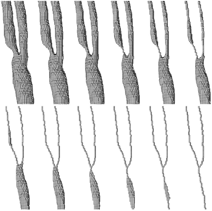 |
| Voxel thinning process. Initial object voxels (top left) and final skeleton (bottom right). |
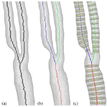 |
| Axis smoothing: (a) Initial voxel skeleton, (b) the initial centroidal lines (circles indicate voxel centres), and (c) the centroidal lines after the smoothing. |
- Obtaining a consistent surface mesh
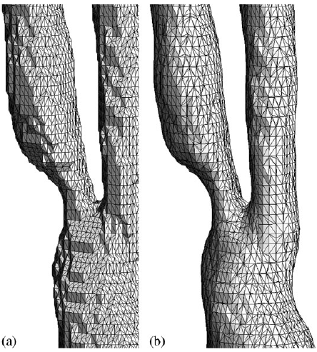 |
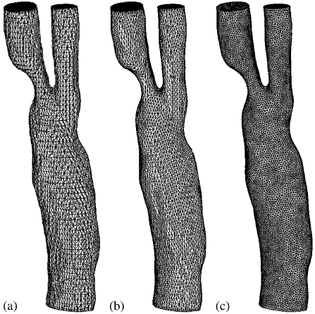
| Surface mesh generated by marching cube methods: (a) standard method and (b) advanced method. |
- Cropping the surface
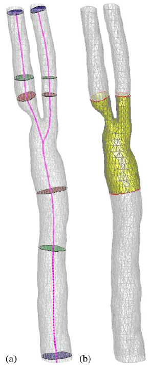 |
| Cropping the surface mesh: (a) automatic determination of inlet/outlet position with different cropping planes and (b) cropped mesh. |
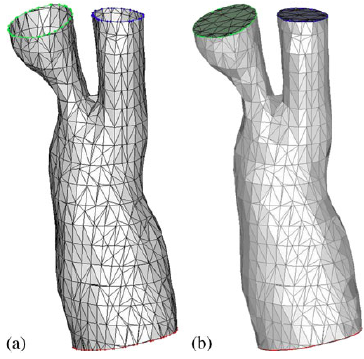 |
| Surface mesh cropping: (a) unclosed mesh after trimming and (b) closed mesh after the triangulation of the inlet and outlet surfaces. |
- Surface mesh cosmetics
 |
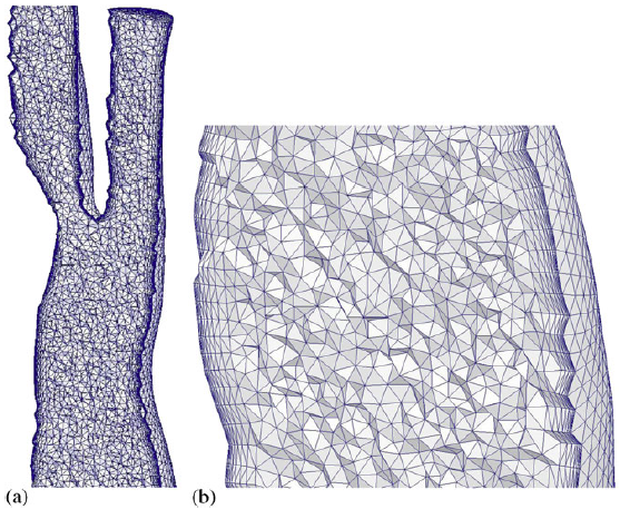
| Surface meshes: (a) mid-cut mesh after before mesh cosmetics; (b) after 10 steps of the Taubin smoothing; and (c) after edge splitting/contraction. |
Volume Meshing
- Boundary layer meshing procedure
- Remove inlet/outlet parts of the surface mesh;
- Decide the number of sub-layers, N, in the boundary-layer mesh and the thickness ratio f;.
- Compute the total thickness;
- Compute inward normals to every point;
- 'Comb' the normals;
- Correct local boundary-layer thickness (shrink or expand) according to the domain crosssectional variations;
- Find positions of the inner surface points (for both wall and ridge points). Smooth the inner surface mesh by Taubing smoothing algorithm;
- To close the inlets/outlets using the stitching method; and
- Generate the quasi-structured, 3D tetrahedral mesh by dividing the prisms into smaller prisms first and then by dividing a smaller prism into three tetrahedra.
- Inner volume mesh
 |
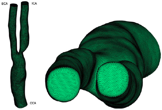
| Volume mesh generated for a carotid artery. |
Example results - final mesh
 |
| Final mesh used for the computation, which consists of 4 126 777 linear tetrahedral elements and 708 191 nodes with 10 structured boundary layers. |
Example results - 3D velocity distribution
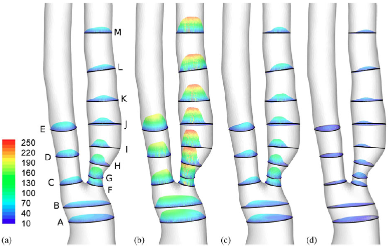 |
| 3D velocity distribution within 13 slices (cm/s): (a) mid accl, (b) peak, (c) mid decel, and (d) dicrotic notch. |
Example results - wall parameter distributions
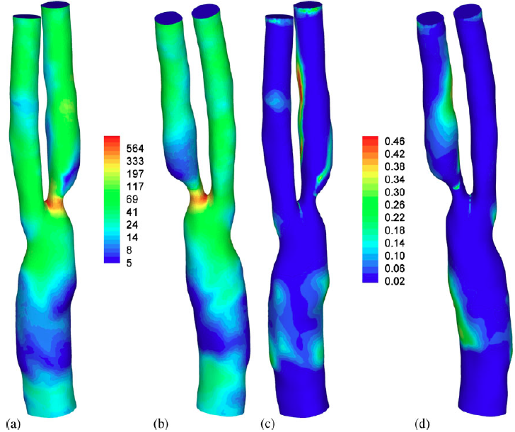 |
| Haemodynamic wall parameter distributions. (a) and (b) Time-averaged WSS (dyne/cm2), (c) and (d) OSI. (a and c) Anterior and (b and d) posterior. |
Fundings
This project was supported by the EPSRC under grants D070554 and H024271. It was also partially supported by the Leverhulme Trust under grant F/00391/R.
Publications
- I. Sazonov, S.Y. Yeo, R.L.T Bevan, X. Xie, R. van Loon, P. Nithiarasu, Modelling pipeline for subject-specific arterial blood flow, International Journal for Numerical Methods in Biomedical Engineering, volume 27, issue 12, December 2011.